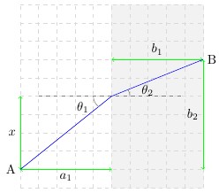
Chapter 1 Lagrangians
Exercise 1: Use Fermat's principle of least time to derive Snell's Law.
Exercise 5: For a three-dimensional elastic medium,the potential energy is
\[ V= \frac{\mathcal{T}}{2}\int \text{d}^3x (\nabla\psi)^2 \]
Where \(\mathcal{T}\) represents the tension/stress; and the kinetic energy is
\[ T= \frac{\rho}{2}\int \text{d}^3x \left(\frac{\partial \psi}{\partial t}\right)^2 \]
Where \(\rho\) represents the mass density.
Use these results, and the functional derivative approach, to show that \(\psi\) obeys the wave equation
\[\nabla^2\psi = \frac{1}{v^2} \frac{\partial^2 \psi}{\partial t^2} \]
Where \(v\) is the velocity of the wave.
Exercise 6: Show that if \[Z_0[J] = exp\left( -\tfrac{1}{2}\int \text{d}^4x\,\text{d}^4y\, J(x)\, \Delta(x-y) J(y) \right)\] where \(\Delta(x) = \Delta(-x)\) then \[\frac{\delta Z_0[J]}{\delta J(z_1)} = -\left[\int \text{d}^4y\,\Delta(z_1-y)J(y)\right] Z_0[J] \]
Chapter 2 Simple harmonic oscillators
Exercise 1: For a one-dimensional harmonic oscillator with annihilation
and creation operators
\[ \hat{a}= \sqrt{\frac{m\omega}{2\hbar}}\left(\hat{x}+\frac{i}{m\omega}\hat{p}\right) \hspace{20pt}
\hat{a}^{†} = \sqrt{\frac{m\omega}{2\hbar}}\left(\hat{x}-\frac{i}{m\omega}\hat{p} \right) \]
show that
\[ [\hat{a},\hat{a}] = 0 \quad\quad [\hat{a}^{†},\hat{a}^{†}] = 0 \quad\quad
[\hat{a},\hat{a}^{†}] = 1\quad\text{and}\quad \hat{H} =
\hbar\omega\big( \hat{a}^{†}\hat{a} + \tfrac{1}{2}\, \big)\]
Exercise 2: For the Hamiltonian \(\hat{H}= \hat{p}^2/2m +
\tfrac{1}{2}m\omega^2\hat{x}^2 + \lambda\hat{x}^4\), where \(\lambda\) is small, show by writing the
Hamiltonian in terms of creation and annihilation operators and using perturbation theory, that the
energy eigenvalues of all the levels are given by
\[ E_n = \big(n+\tfrac{1}{2}\big)\hbar\omega +\frac{3\lambda}{4}\left(\frac{\hbar}{m\omega}\right)^2
(2n^2+2n+1) \]
Exercise 4: Using \(\hat{a}\ket{0}=0\) and the annihilation and creation operators \[ \hat{a} = \sqrt{\frac{m\omega}{2\hbar}}\left(\hat{x}+\frac{i}{m\omega}\hat{p}\right) \hspace{20pt} \hat{a}^{†} = \sqrt{\frac{m\omega}{2\hbar}}\left(\hat{x}-\frac{i}{m\omega}\hat{p}\right) \] together with \[ \bra x \hat{p} \ket{\psi} = -i\hbar\frac{\text{d}}{\text{d}x}\braket{x|\psi} \] show that \[ \left(x+\frac{\hbar}{m\omega}\frac{\text{d}}{\text{d}x}\right) \braket{x|0} = 0 \] and hence \[ \braket{x|0} = \left(\frac{m\omega}{\pi\hbar}\right)^{1/4} e^{-m\omega x^2/2\hbar} \]
Chapter 3 Occupation number representation
Exercise 2: Show that for a simple harmonic oscillator
(a) \( \big[ \hat{a}, (\hat{a}^{†})^n \big] = n(\hat{a}^{†})^{n-1}\)
(b) \( \bra{0} \hat{a}^n(\hat{a}^{†})^m \ket{0} = n!\,\delta_{nm}\)
(c) \( \bra{m} \hat{a}^{†} \ket{n} = \sqrt{n+1}\,\delta_{m,n+1}\)
(d) \( \braket{m|\hat{a}|n} = \surd{n}\,\delta_{m,n-1}\)
Exercise 3: The three-dimensional harmonic oscillator is described by
the Hamiltonian
\[ \hat{H} =\frac{1}{2m}(\hat{p}_1^2 + \hat{p}_2^2 + \hat{p}_3^2) +\tfrac{1}{2}m\omega^2(\hat{x}_1^2 +
\hat{x}_2^2 + \hat{x}_3^2)\]
Define creation operators \(\hat{a}^{†}_1\), \(\hat{a}^{†}_2\), and \(\hat{a}^{†}_3\)
so that
\(\big[\hat{a}_i,\hat{a}^{†}_j\big]=\delta_{ij}\) and show that \(\hat{H} = \hbar\omega\sum_{i=1}^3
(\tfrac{1}{2}+\hat{a}^{†}_i \hat{a}_i)\).
Angular momentum can be defined as
\( \hat{L}^i =-i\hbar\epsilon^{ijk}\hat{a}^{†}_j \hat{a}_k\) where \(\epsilon^{ijk}\)
is the Levi-Civita symbol, so that for example \(\hat{L}^3 = -i\hbar(\hat{a}^{†}_1\hat{a}_2 -
\hat{a}^{†}_2\hat{a}_1)\).
Define new creation operators
\[ \hat{b}^{†}_1 = -\frac{\,1}{\surd{2}}(\hat{a}^{†}_1 + i\hat{a}^{†}_2) \hspace{20pt}
\hat{b}^{†}_0 = \hat{a}^{†}_3 \hspace{20pt} \hat{b}^{†}_{-1} = \frac{\,1}{\surd{2}}
(\hat{a}^{†}_1 - i\hat{a}^{†}_2) \]
and show that \(\big[\hat{b}_i,\hat{b}^{†}_j \big]=\delta_{ij}\), the Hamiltonian is \(\hat{H}=
\hbar\omega\sum_{m=-1}^1 (\tfrac{1}{2}+\hat{b}^{†}_m\hat{b}_m)\) and \(\hat{L}^3= \hbar\sum_{m=-1}^1
m\hat{b}^{†}_m \hat{b}_m\)
Exercise 4: Since for fermions we have that \(\hat{c}^{†}_1
\hat{c}^{†}_2 \ket{0}= -\hat{c}^{†}_2 \hat{c}^{†}_1 \ket{0}\), then the state \(\ket{11}\)
depends on which fermion is added first. If we put the first fermion into the state \(\psi_i(r_1)\) and
the second fermion into the state \(\psi_j(r_2)\), a representation for \(\ket{11}\) is
\[ \Psi(r_1,r_2) = \frac{\,1}{\surd{2}} \Big[\psi_1(r_1)\psi_2(r_2) - \psi_2(r_1)\psi_1(r_2)\Big] \]
Show that a generalization of this result for \(N\) fermions is \(\Psi(r_1\, ...\, r_N)\), which can be
written out as
\begin{equation*}
\frac{1}{\sqrt{N!}}\,
\begin{vmatrix}
\,\,
\psi_1(r_1) & \psi_2(r_1) & ... & \psi_N(r_1)\\
\psi_1(r_2) & \psi_2(r_2) & ... & \psi_N(r_2)\\
\cdot & \cdot & \cdot & \cdot\\
\cdot & \cdot & \cdot & \cdot\\
\psi_1(r_N) & \psi_2(r_N) & ... & \psi_N(r_N)
\,\,
\end{vmatrix}
\end{equation*}
This expression is known as a Slater determinant.
Chapter 4 Making the second quantization work
Exercise 1: We can define a generalized commutator
\(\big[\hat{A},\hat{B}\big]_{\zeta}\) as
\[ \big[\hat{A},\hat{B}\big]_{\zeta} = \hat{A}\hat{B} - \zeta\hat{B}\hat{A} \]
so that \(\zeta=1\) yields \(\big[\hat{A},\hat{B}\big]_{\zeta}=\big[\hat{A},\hat{B}\big]\) for bosons
and \(\zeta=-1\) yields \(\big[\hat{A},\hat{B}\big]_{\zeta}=\big\{\hat{A},\hat{B}\big\}\) for fermions,
the generalized commutation relations can then be written
\[ \big[\hat{\psi}(\textbf{x}), \hat{\psi}^{\dagger}(\textbf{y})\big]_{\zeta} = \delta^{(3)}
(\textbf{x}-\textbf{y}) \]
and
\[ \big[\hat{\psi}(\textbf{x}), \hat{\psi}(\textbf{y})\big]_{\zeta} = 0 \]
Using the argument given in the text (\(\S 4.3^*\)) and the generalized commutator show that
\(\hat{V}_{wrong}\) yields the same result for both bosons and fermions.
Exercise 3: Evaluate the eigenvalues and eigenvectors of the
Hubbard Hamiltonian
\[\begin{equation*}
\hat{H}=
\begin{pmatrix}
\,\,
U & -t & t & 0\\
-t & 0 & 0 & -t\\
t & 0 & 0 & t\\
0 & -t & t & U
\,\,
\end{pmatrix}
\end{equation*}\]
(a) What are the energy eigenvalues in the limit \(t=0\) ?
(b) How do these energy levels change as \(t\neq 0\) in the limit \(t/U << 1\) ?
Chapter 5 Continuous systems
Exercise 2: Show that Poisson brackets anticommute
\[ \{A,B\}_{PB} = -\{B,A\}_{PB} \]
and also satisfy the Jacobi identity
\[ \{ \{A,B\}_{PB}, C\}_{PB} + \{ \{C,A\}_{PB}, B\}_{PB} + \{ \{B,C\}_{PB}, A\}_{PB} = 0 \]
and show that the quantum mechanical commutators also have the same properties.
Exercise 4: The Lagrangian for a free particle is
\(L= -mc^2/\gamma \). Find an expression for \(L\), \(p\) and \(H\) when \( v\lt\lt c \).
Exercise 6: Use the Lagrangian \[ L=-\frac{mc^2}{\gamma} +
q\textbf{A} \boldsymbol{\cdot} \textbf{v }- qV \]
for a free particle of charge \(q\) and mass \(m\) in an electromagnetic field to derive the Lorentz force, i.e.
\[ \frac{\text{d}}{\text{d}\textit{t}}(\gamma m\textbf{v}) =
q (\textbf{E} + \textbf{v} \boldsymbol{\times}\textbf{B}) \]
Exercise 9: Show that \(\partial_{\mu}F^{\mu\nu}=J^{\nu}\)
reduces to two of Maxwell's equations, and that the other two can be generated from the equation
\[ \partial_{\lambda}F_{\mu\nu} + \partial_{\mu}F_{\nu\lambda} + \partial_{\nu}F_{\lambda\mu} = 0 \]
Chapter 6 A first stab at relativistic quantum mechanics
Exercise 1: Show that the Lagrangian density \(\mathcal{L}\) given by
\[ \mathcal{L} = \frac{1}{2}\big(\partial_\mu\phi\big)^2 - \frac{1}{2}m^2\phi^2 \] yields the Klein-Gordon equation when
using the Euler-Lagrange equation. Also derive expressions for the momentum \(\pi= \partial{\mathcal{L}}/\partial\dot\phi\)
and the Hamiltonian density \(\mathcal{H} = \pi\dot\phi - \mathcal{L}\) for this Lagrangian.
Chapter 7 Examples of Lagrangians, or how to write down a theory
Exercise 3: Show that the equations of motion following from the Lagrangian
\[ \mathcal{L} = \frac{1}{2}(\partial_{\mu}\phi_1)^2 - \frac{1}{2}m^2\phi_1^2 + \frac{1}{2}(\partial_{\mu}\phi_2)^2 -
\frac{1}{2}m^2\phi_2^2 - g(\phi_1^2+\phi_2^2)^2 \]
are the coupled equations
\[ \partial_{\mu}\partial^{\mu}\phi_1 + m^2\phi_1 + 4g\phi_1(\phi_1^2+\phi_2^2) = 0 \]
\[ \partial_{\mu}\partial^{\mu}\phi_2 + m^2\phi_2 + 4g\phi_2(\phi_1^2+\phi_2^2) = 0 \]
Exercise 4: Show that the equation
\[ \mathcal{L} = \frac{1}{2}\big(\partial_\mu\phi\big)^2 - \frac{1}{2}m^2\phi^2 \]
is equivalent to
\[ \mathcal{L} = \frac{1}{2}\dot\phi^2 - \frac{1}{2}\big(\boldsymbol\nabla \phi\big)^2 - \frac{1}{2} m^2\phi^2 \]
Show that
\[ \pi = \frac{\partial\mathcal{L}}{\partial\dot\phi} =\dot{\phi} \]
and
\[ \mathcal{H} = \frac{1}{2}\dot\phi^2 + \frac{1}{2}\big(\boldsymbol\nabla \phi\big)^2 + \frac{1}{2} m^2\phi^2 \]
Define the quantity
\[ \Pi^{\mu} = \frac{\partial\mathcal{L}}{\partial(\partial_\mu \phi)} \]
and show that \(\Pi^{\mu}=\partial^{\mu}\phi\) and \(\Pi^0=\pi=\dot{\phi}\)
I have posted a few solutions to give a flavour of the book. A more complete set of solutions is available at pdfcoffee. The authors Nischal Dwivedi and Sandeep Joshi have more expertise than I do; and I'm indebted to them for helping me to understand the subject so far.
J D Cain